ergodic.io - Differentiable Thomson scattering for near real-time plasma diagnostics

We applied reverse-mode automatic differentiation (AD) to Thomson-scattering data analysis for laser-plasma and inertial fusion experiments. By making the entire diagnostic model differentiable with JAX and running on GPUs, we achieved a >140x speedup over finite-differencing approaches. This is fast enough for near real-time use during experiments — and because reverse-mode AD scales independently of the number of parameters, we can now fit with O(1000) free parameters, enabling direct measurement of electron velocity distribution functions from angularly resolved Thomson scattering data.

[Publication on Machine Learning: Science and Technology]

A.L. Milder, A.S. Joglekar, W. Rozmus, and D.H. Froula, Mach. Learn.: Sci. Technol. 5, 015026 (2024)

The idea: make diagnostic fitting differentiable

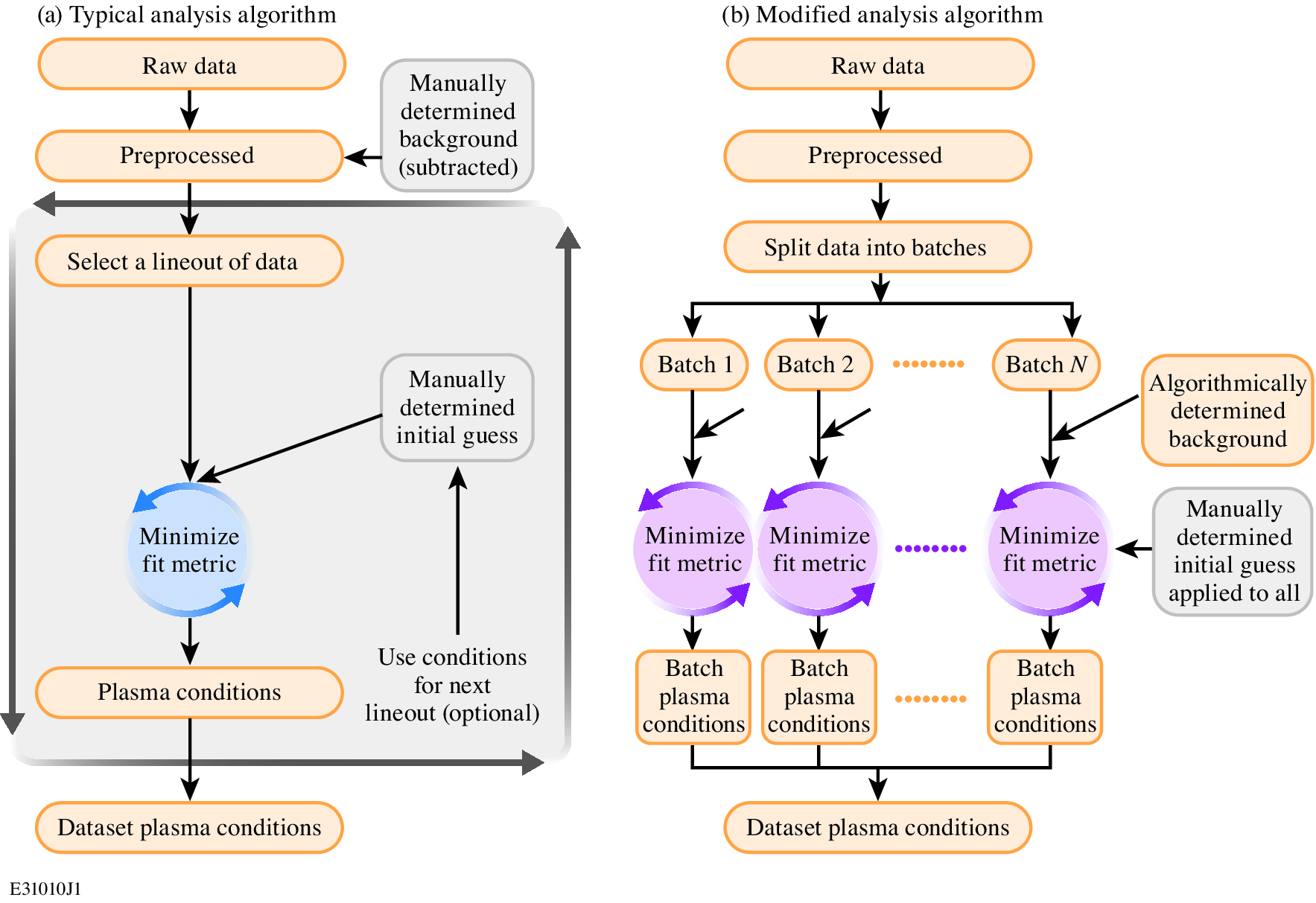
Parameter estimation in experimental plasma physics involves matching a physics-based model to observed data — effectively an optimization problem. The standard approach uses finite differencing to compute gradients, which requires two function evaluations per parameter and scales linearly with parameter count. This makes high-dimensional fits and batch processing prohibitively expensive.

We rewrote the Thomson-scattering diagnostic model as a fully differentiable program using JAX. Reverse-mode AD computes the gradient with respect to all parameters in a single backward pass, regardless of how many there are. Combined with GPU acceleration and a batched workflow that processes multiple lineouts simultaneously, this eliminates the manual loop-over-lineouts bottleneck that has defined Thomson-scattering analysis for decades.

Comparison of the typical manual analysis algorithm (left) with the AD-optimized batched workflow (right). Grey boxes indicate manual steps; orange boxes are automated. The batched approach removes user intervention and processes entire datasets with a single set of initial conditions.

The physics: Thomson scattering as a diagnostic

Thomson scattering measures plasma conditions — electron density, temperature, ionization state, flow velocity — by analyzing the spectrum of laser light scattered from plasma fluctuations. The scattered power depends on the spectral density function, which in turn depends on the electron and ion velocity distribution functions and the dielectric response of the plasma. The model maps physical parameters to a predicted spectrum; fitting inverts this to extract plasma conditions from data.

The diagnostic model includes scattering geometry, amplitude normalizations for different spectral features, convolution with instrumental effects, and optionally plasma gradients across the scattering volume. For non-Maxwellian distributions, the electron susceptibility must be computed numerically for each spectrum evaluation, making the forward model expensive — and making efficient gradient computation critical.

Key technical choices

Batched fitting. Rather than fitting one lineout at a time, the data is split into batches of 6 lineouts whose combined loss is minimized simultaneously. This reduces the number of minimizations while only marginally increasing the cost per batch, since AD makes the gradient cost nearly independent of parameter count.

Automated background handling. Instead of manually subtracting background, it is determined algorithmically and added to the model during fitting, preserving Poisson statistics for proper uncertainty estimation.

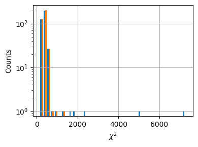
L-BFGS-B optimization with normalized parameters (scaled between user-supplied bounds) for stable convergence. Bad fits are automatically detected via a chi-squared threshold and refit using neighboring solutions as initial conditions.

Performance: >140x speedup

Switching from finite differencing on CPU to reverse-mode AD on GPU produces a two-order-of-magnitude speedup in gradient computation. AD alone provides roughly 10x by eliminating the per-parameter scaling; the GPU provides another 10x through hardware acceleration.

Fitting time versus number of parameters for finite differencing (blue) and automatic differentiation (red), on CPU (solid) and GPU (dashed). AD+GPU is consistently two orders of magnitude faster and scales nearly flat with parameter count.

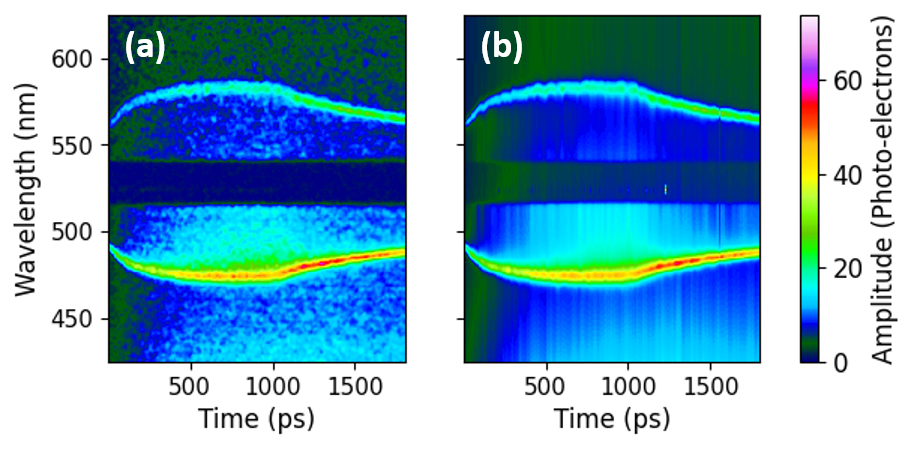
Applied to a temporally resolved Thomson-scattering dataset, the AD workflow analyzed 360 lineouts (1 pixel per lineout) in 11.2 minutes including postprocessing and refitting. The previous finite-differencing approach required 90 minutes for 20 lineouts — a 144x acceleration per lineout.

Raw Thomson-scattering data (left) compared to the best-fit reconstruction (right). The fit reproduces the evolution of peak separation, width, and inter-peak structure across the full temporal range.

Extracted plasma conditions with uncertainty

With per-pixel resolution, we extracted electron density, temperature, and super-Gaussian order as continuous functions of time — resolving the full plasma evolution from laser heating through cooling after the drive turns off.

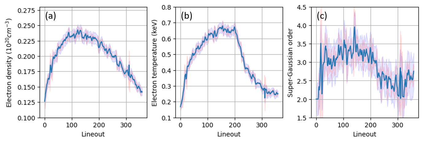
Plasma conditions extracted from the full dataset: (a) electron density, (b) electron temperature, (c) super-Gaussian order versus lineout number. Blue shaded regions show 3-sigma uncertainty from the Hessian; red shaded regions show 3-sigma from a 5-pixel moving standard deviation.

Two independent uncertainty estimates — the Hessian-based covariance (computed efficiently via AD second derivatives) and a moving-window standard deviation over the diagnostic resolution unit — are in good agreement, validating both approaches.

Examples of (a) a good fit where the model reproduces spectral features within Poisson uncertainty, and (b) a bad fit where the minimizer converged to a local minimum with visible discrepancies in peak width and height. Data is shown in blue, best fit in orange.

The automated refitting step reduced the number of bad fits (where the minimizer converged to a local minimum) from 5 out of 360 to nearly zero.

Histogram of the fit metric before (blue) and after (orange) refitting, showing that most bad fits are recovered.

New capability: measuring electron distribution functions

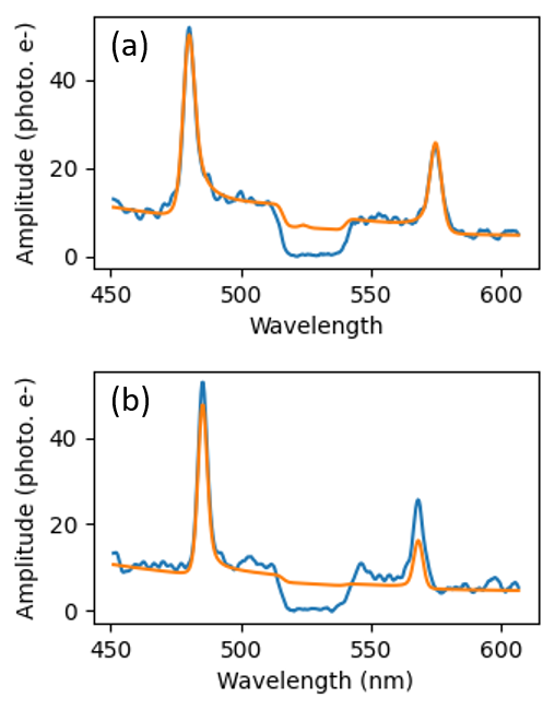
Because reverse-mode AD removes the parameter-count bottleneck, we can now represent the electron velocity distribution function as a set of free parameters — over 256 points — and fit it directly from angularly resolved Thomson scattering data. This was previously computationally prohibitive: earlier analysis required at least 8 hours for 64 distribution function points. The AD approach completes the same task in 15.4 minutes with 4x the resolution, a 30x speedup.

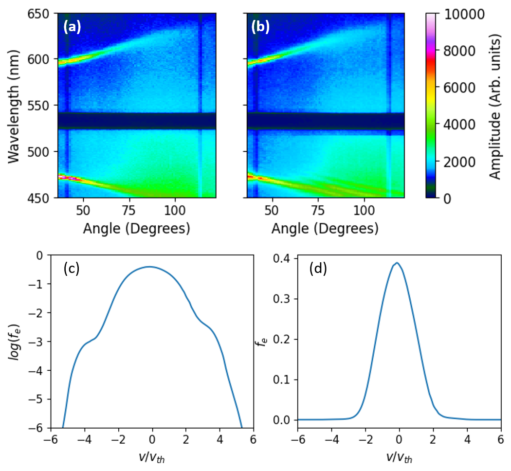
Angularly resolved Thomson scattering: (a) raw data as a function of wavelength and angle, (b) best-fit reconstruction, (c) recovered electron distribution function on a logarithmic scale, (d) on a linear scale.

This is a qualitatively new measurement capability — direct interrogation of the particle velocity distribution function from scattering data, enabled entirely by the efficiency of differentiable programming.

How it was done

Framework: JAX for automatic differentiation and GPU compilation via XLA
Optimizer: SciPy L-BFGS-B with parameter normalization between user-supplied bounds
Batch size: 6 lineouts per batch (optimal tradeoff between speed and convergence)
Hardware: A10G Tensor Core GPU and AMD EPYC 7R32 CPU (AWS)
Dataset: 360 temporal lineouts of Thomson-scattering data from a laser-plasma experiment
ARTS fit: 256-point distribution function, single angularly resolved measurement, 15.4 minutes
Code: Open source at github.com/ergodicio/inverse-thomson-scattering

Broader implications

This approach generalizes beyond Thomson scattering. Any model-based diagnostic — interferometry, proton radiography, spectroscopy — that currently relies on finite-differencing or manual fitting can be rewritten as a differentiable program. The recipe is the same: implement the forward model in an AD framework, batch the data, and let reverse-mode gradients handle the scaling. The result is faster analysis, higher resolution, rigorous uncertainty quantification, and the ability to fit models with far more parameters than previously feasible — including embedding neural networks to represent missing physics.