Discovering novel physics using differentiable kinetic simulations
We built a fully differentiable kinetic plasma solver and used it to discover a previously unknown physical mechanism: nonlinear plasma wavepackets that persist far longer than expected when a second wavepacket is driven in the wake of a first. The optimization found this on its own — we just asked it to maximize electrostatic energy and non-Maxwellian-ness.
This article was featured in the Journal of Plasma Physics for most of 2023. Published under CC-BY 4.0.
A.S. Joglekar and A.G.R. Thomas, J. Plasma Phys. 88, 905880608 (2022)
The idea: close the loop on simulation with gradients
Computational plasma physics typically works in an open loop — a researcher picks parameters, runs a simulation, interprets the output, and repeats. We replaced this manual cycle with a closed-loop, gradient-based optimization by making the entire simulation differentiable using JAX.
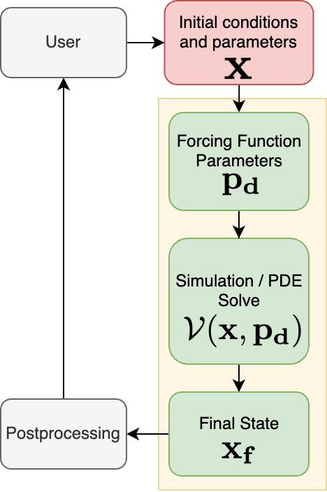
The progression from (a) to (d) above is the key conceptual contribution. In the final step, a neural network generates the forcing function parameters given the physics — and the entire pipeline (neural net + PDE solver + cost function) is differentiated end-to-end to train the network. This is unsupervised: no labeled data is needed, only a physics-informed objective.
The physics: what happens when wavepackets interact?
Large-amplitude electrostatic waves in plasma trap electrons, forming nonlinear wavepackets (finite-length analogues of Bernstein-Greene-Kruskal modes). These wavepackets are relevant to stimulated Raman scattering in inertial confinement fusion. Prior work (Fahlen et al. 2009) showed that isolated wavepackets self-destruct through a process called etching — resonant electrons transit through the slower-moving wave, restoring a Maxwellian distribution at the rear, which re-enables Landau damping.
We asked: what happens when a second wavepacket is driven in the presence of a first? Rather than scan a 4D parameter space by brute force, we posed this as an optimization problem. Given the wavenumber of the first wavepacket and the excitation time of the second, we trained a neural network to learn the optimal spatial location and frequency shift for the second wavepacket.
The cost function: domain-specific and unsupervised
We designed a loss function combining two physics-motivated terms:
- Electrostatic energy — we want the waves to persist, so we maximize the time-integrated electric field energy
- Kinetic entropy deviation — we want nonlinear kinetic effects, so we maximize the deviation of the distribution function from a local Maxwellian (a measure of non-Maxwellian-ness)
The neural network weights were optimized to minimize the combined loss using gradients backpropagated through the entire Vlasov-Poisson-Fokker-Planck simulation. No target data, no supervision — just physics objectives.
The discovery: superadditive, long-lived wavepackets
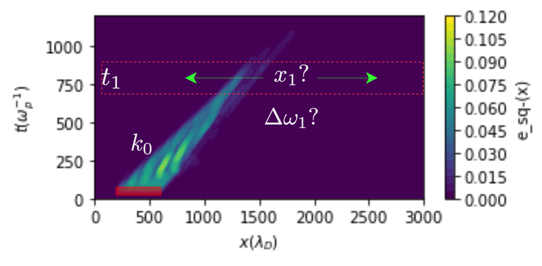
The optimization discovered a superadditive effect. A wavepacket driven alone damps away through the etching process. But when a second wavepacket is driven at the right place and time, the combined system retains far more energy than the sum of the individual wavepackets.
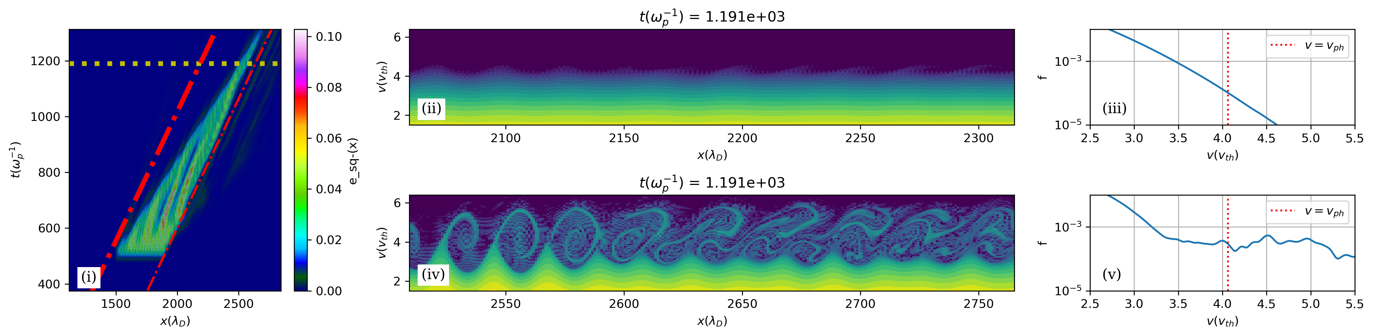
The phase-space analysis reveals the mechanism. In an isolated wavepacket, the rear returns to a Maxwellian and Landau damping resumes (left panel below). When both wavepackets are present, detrapped electrons streaming from the first wavepacket arrive at the rear of the second and flatten the distribution function at the phase velocity — suppressing Landau damping and preventing etching (right panel below).
| Isolated wavepacket | Both wavepackets present |
|---|---|
 |
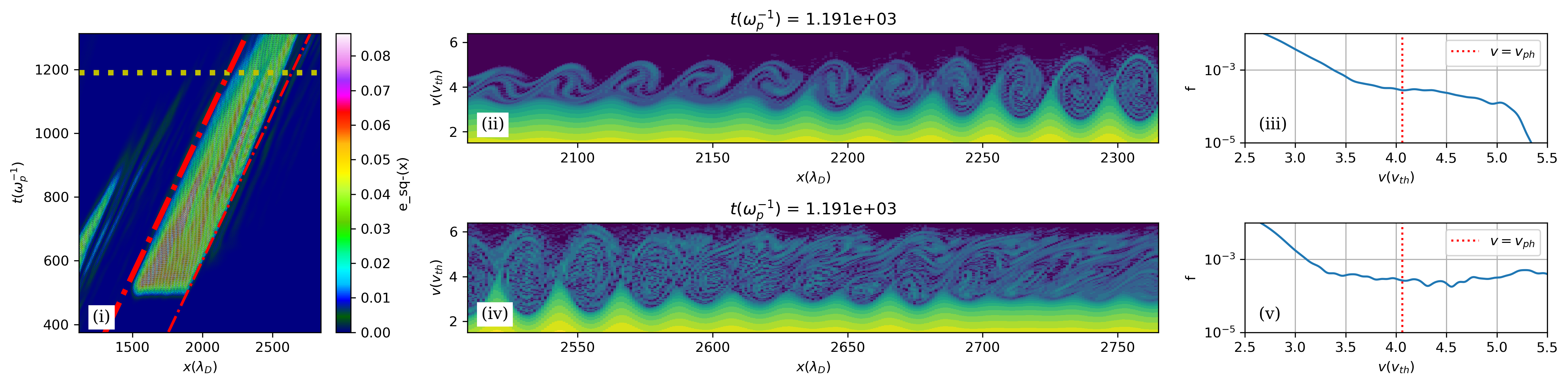 |
The left panel shows an isolated second wavepacket: the rear of the wave has returned to a Maxwellian (no trapping activity), and Landau damping is etching the wave away. The right panel shows the same wavepacket in the presence of a pre-existing first wavepacket: there is significant trapped-particle activity at the rear, the distribution is flattened at the phase velocity, and the wave persists far longer.
Learned functions: what the neural network found
The trained neural network provides continuous, physically interpretable functions for the optimal parameters:
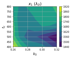
Resonant spatial location — The optimal excitation location tracks the phase velocity of resonant electrons, roughly following the relationship x ~ v_ph * t. Waves with larger wavenumbers have smaller phase velocities, so the resonant location decreases with increasing wavenumber.
| Learned spatial location | Space-time locus for k=0.28 |
|---|---|
 |
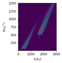 |
The locus of points (right) suggests a critical space-time radius within which collisional relaxation has not yet occurred and nonlinear effects can be exploited.
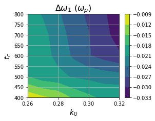
Frequency shift — The learned frequency shift is negative and a few percent in magnitude — consistent with known nonlinear frequency shifts. It increases in magnitude with wavenumber because higher-k waves interact with more particles.
How it was done
- Solver: Differentiable Vlasov-Poisson-Fokker-Planck in 1D-1V, built in JAX with spectral methods and a 6th-order Hamiltonian integrator
- Grid: 6656 spatial points, 160 velocity points, 1200 timesteps
- Neural network: 2-layer MLP (8 nodes wide, Leaky-ReLU activations, tanh output)
- Training: 35 input samples across the (k0, t1) space, 60 epochs, ~150 GPU-hours on NVIDIA T4
- Memory: Gradient checkpointing at every timestep to fit on a single GPU
The gradient-based approach reduced this from a 4D brute-force scan to a 2D search + 2D gradient descent, escaping the curse of dimensionality.
Broader implications
This workflow is not limited to differentiable simulations. The PDE solver in the loop can be replaced by any auto-differentiable model of a physical system — including a pre-trained neural network emulator. The framework applies anywhere you can pose a physics question as an optimization problem and differentiate through the forward model.