Differentiable programming for plasma physics
Differentiable programming applies automatic differentiation to numerical solvers, turning any simulation into a component of a gradient-based optimization pipeline. In this invited review, we argue that this is not just a speedup trick but a unifying computational framework for plasma physics. We demonstrate this through four applications: discovering novel kinetic physics, learning fluid closures for kinetic effects, accelerating experimental Thomson-scattering diagnostics, and inverse-designing structured laser pulses. Each uses the same infrastructure — reverse-mode AD through a physics solver — but addresses a fundamentally different type of problem.
This paper was an invited contribution to Physics of Plasmas.
A.S. Joglekar, A.G.R. Thomas, A.L. Milder, K.G. Miller, J.P. Palastro, and D.H. Froula, Phys. Plasmas 32, 022501 (2025)
The framework: from manual iteration to function learning
The core idea is a progression in how computational physics is done. Traditional workflows are open-loop: pick parameters, run a simulation, analyze, repeat. Differentiable programming closes this loop by providing exact gradients of a scalar objective with respect to all inputs — at a cost that is independent of the number of parameters.
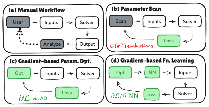
The key step is from (c) to (d). In stage (d), a neural network generates parameters for a physics solver. The chain rule propagates gradients through the network, the solver, and the objective — the network learns continuous functional relationships through the physics. No labeled training data is needed, only a physics-motivated cost function. The four applications in this paper span stages (c) and (d).
Where differentiable simulation fits
Differentiable simulation is distinct from surrogates, PINNs, and neural operators in a crucial way: the physics-based solver produces the solution, and any learned component merely generates parameters or closures for that solver. The governing equations — not a loss penalty or training distribution — enforce physical constraints. This has practical consequences for interpretability, conservation, and extrapolation that show up across all four applications.
Application 1: Discovering novel kinetic physics
We built a differentiable Vlasov-Poisson-Fokker-Planck solver and trained a neural network to learn optimal wavepacket excitation strategies by maximizing electrostatic energy and non-Maxwellian-ness. The optimization discovered a previously unknown superadditive regime: two interacting wavepackets sustain electrostatic energy far longer than either would alone.
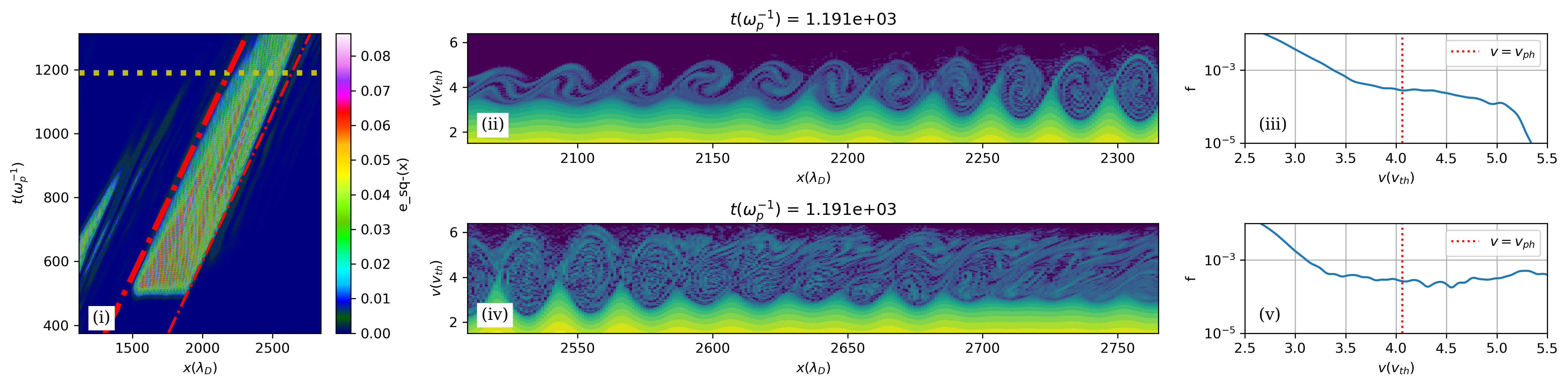
The learned functions recovered physically interpretable scalings — optimal excitation location tracks the phase velocity, frequency shifts match trapped-particle theory — all without imposing these relationships. The neural network discovered mechanisms, not just parameters.
Full details: Discovering novel physics using differentiable kinetic simulations
Application 2: Learning kinetic closures for fluid simulations
Nonlinear Landau damping introduces spatiotemporal nonlocality that no local fluid closure can capture. We introduced a hidden dynamical variable into a differentiable fluid solver, representing the resonant electron population. Its growth rate — the only unknown — was learned by a 160-parameter neural network trained through indirect supervision: comparing fluid and kinetic predictions of density mode amplitudes, with gradients backpropagated through the entire simulation.
| Vlasov simulation (truth) | Learned hidden-variable closure |
|---|---|
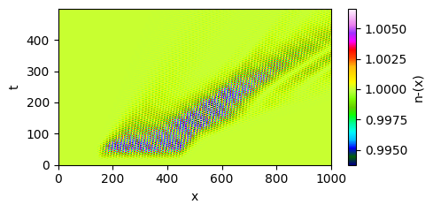 |
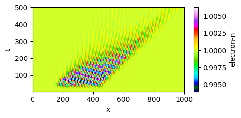 |
Trained only on single-wavelength periodic boxes, the model generalizes to wavepackets in domains 100x larger with open boundaries — reproducing etching that a local closure misses entirely. The physics encoded in the transport equation provides the generalization; the network just learns a coefficient.
Full details: Deep learned closure model for nonlinear Landau damping
Application 3: Accelerating Thomson-scattering diagnostics
Reverse-mode AD transforms Thomson-scattering analysis from a slow, serial, manual process into a fast, batched, automated one. The full diagnostic model — spectral density function, susceptibility integrals, instrumental convolution — was implemented in JAX, making it differentiable with respect to all plasma and instrumental parameters.
The speedup enables per-pixel analysis of entire datasets, Hessian-based uncertainty quantification at negligible additional cost, and — most importantly — fitting electron velocity distribution functions with over 256 free parameters. This transforms Thomson scattering from measuring bulk parameters into probing kinetic physics directly.
Full details: Differentiable Thomson scattering for near real-time plasma diagnostics
Application 4: Inverse design of spatiotemporal laser pulses
Discovery asks “what physics emerges from optimized inputs?” Inverse design asks the converse: “what inputs produce desired physics?” We applied gradient-based optimization to design structured laser pulses — with coupled spatial and temporal features — that achieve target far-field behavior.
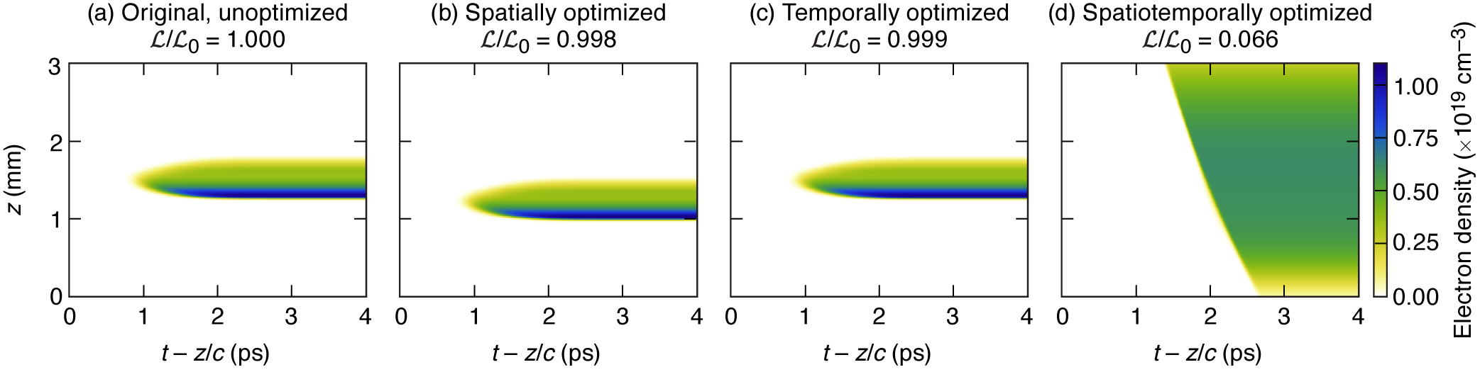
The framework was applied to three problems. The most striking is generating a uniform plasma column through ionization in hydrogen gas. Purely spatial optimization reduces the loss by 0.2%. Purely temporal optimization: 0.1%. Full spatiotemporal optimization: 93%. Coupled space-time structure provides capabilities fundamentally inaccessible to either dimension alone.
The optimized pulse exhibits complex near-field structure — radially varying central frequency, duration, and amplitude with chromatic focusing — that would never emerge from forward design. The optimization also discovered a flying-focus configuration with superluminal (1.14c) intensity peak, entirely autonomously.
Implementation across applications
All four applications use reverse-mode AD through JAX. The key enabling techniques are shared:
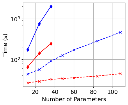
- Reverse-mode AD provides gradients at O(1) cost regardless of parameter count — critical for problems ranging from 10 parameters (Thomson scattering per lineout) to 1000+ (distribution function fitting, neural network weights)
- Gradient checkpointing trades compute for memory, reducing storage from O(T) to O(sqrt(T)) timesteps — essential for the long kinetic and fluid simulations
- Neural networks as function generators — the network does not replace the physics; it generates parameters for a first-principles solver, ensuring interpretability and conservation
- Physics-motivated loss functions — no labeled data needed; objectives are defined in terms of physical quantities (electrostatic energy, mode amplitudes, spectral fit residuals, target far-field profiles)
Broader implications
The same AD infrastructure that accelerates a diagnostic also discovers nonlinear wave interactions and learns multiscale closures. This is not a coincidence — all are inverse problems posed within physics-based models. As differentiable programming tools mature, combining them with symbolic regression offers a path toward automated hypothesis generation: optimization identifies candidate mechanisms, and symbolic analysis distills them into interpretable mathematical relationships.